A common problem in biomechanics is determining what cutoff frequency to use for filtering collected positional data. We want to filter out the noise while retaining as much of the signal as possible, including the sharp peaks and valleys where a lot of the interesting information is. Often data is collected in a lab setting where the conditions are controlled, other research studies can be used as guidance, and a single cutoff frequency is appropriate for all the collected trials.
However, a current project I’m working on uses computer vision to track the position of a barbell that can be used in a variety of settings. The solution is designed to track the two main Olympic lifts (Snatch, Clean and Jerk) which each have distinct characteristics in regard to velocity, acceleration, and duration. Additionally, I use two different tracking algorithms depending on if there is a blue target plate on the bar (for better tracking) or if I’m tracking the barbell plates directly. Differences in lighting, background, and distance from the object can also affect the tracking. I need to be able to determine the appropriate cutoff frequency for each capture, given these factors, that still results in consistent, reliable data trial to trial.
A popular method to determine the appropriate cutoff frequency is residual analysis (Winter 2009). There are some resources available to explain the concept but I found they often didn’t have applied examples so I decided to write this post and show my process.
The raw tracking for three distinct cases are shown below. (1) A “clean” tracking the plates directly, (2) A “snatch” tracking the plates directly, and (3) a “snatch” tracking the blue target disk. The same video was used for case (2) and (3) so the difference in results based on the tracking method and subsequent filtering could be compared.

- Clean – Plate Tracking
2. Snatch – Plate Tracking
3. Snatch – Target Tracking
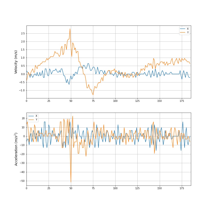
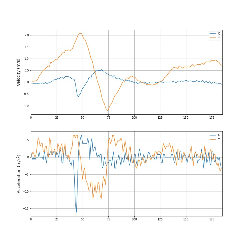
Each video has a distinct signal and noise profile. If we calculate the velocity/acceleration directly from the raw signals, we get the series data shown below. The series data, especially acceleration, is volatile because small tracking errors magnify during differentiation and it’s difficult to discern useful information regarding the signal. Since the noise is clearly different in the two plots below, the cutoff frequencies need to be different too.
RESIDUAL ANALYSIS
The ideal cutoff frequency is determined from a residual plot that shows the difference between the raw and filtered data over a range of cutoff frequencies. “Biomechanics and Motor Control of Human Movement” by Winter was the primary reference used for this analysis and goes deeper into the technical details behind it. All filtering was done in Python with a second-order Butterworth filter, filtered forward and backward, to result in a zero-lag, fourth-order filter.

Steps to create the residual plot and calculate the cutoff frequency:
- 1) Filter the raw data at each frequency over the test range. Based on some past analysis, I thought the ideal frequency would be between 2.5 and 6 Hz so I tested every frequency between 1 and 10 Hz at 0.1 Hz intervals
- 2) After filtering at each frequency, calculate the root mean squared error (RMSE) between the raw and filtered data points.
- 3) The calculated RMSE value for each frequency is plotted on the vertical axis with the frequencies on the horizontal axis (blue solid line).
- 4) Residual plots generally increase slowly at higher frequencies before sharply increasing when the signal starts to be affected. A line is plotted through the tail of the residual plot to its Y-intercept (gray dashed line).
- 5) The Y-intercept is considered to be the threshold value (red dashed line). The frequency at which the RMSE exceeds the threshold value is chosen as the cutoff frequency for the analysis.


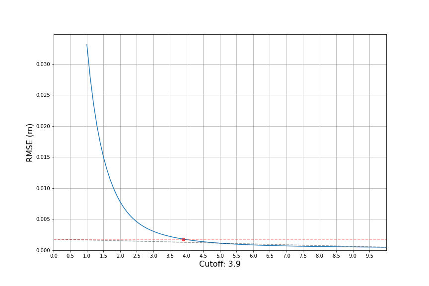
The calculated cutoff frequencies follow what we would intuitively expect based on the differences between the captures. The clean has the lowest calculated frequency because it’s both the slowest movement and is tracked directly by the plates. The snatch video using the target tracking had the highest calculated cutoff frequency because it’s a faster movement and is tracked using the blue target disk which is less noisy.
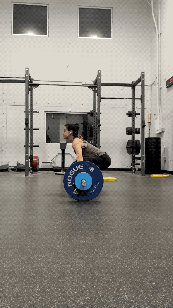
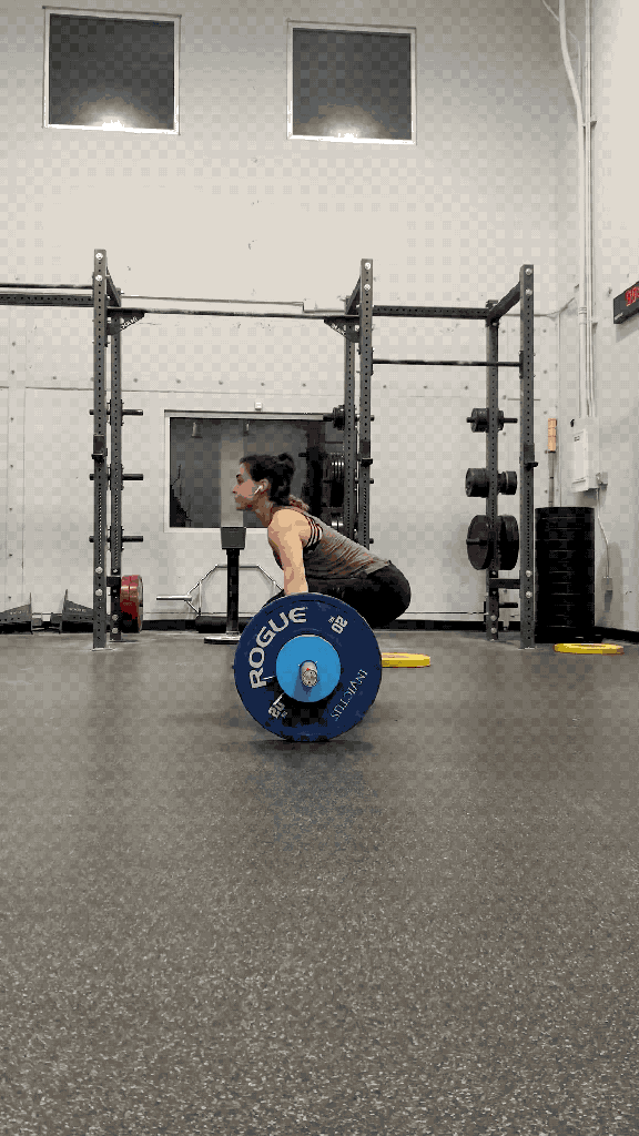
When superimposed back over the videos, the filtered trajectories look smooth and visually follow the path of the barbell.
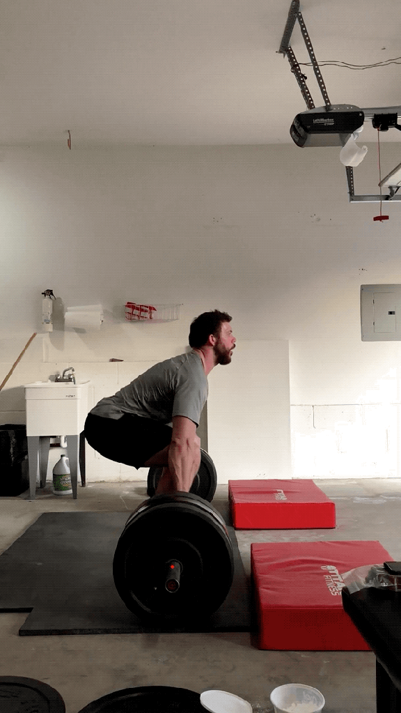
Clean – Plate Tracking

Snatch – Plate Tracking

Snatch – Target Tracking
The effect of filtering on the calculated velocities and accelerations is significant. The plots are much smoother and the characteristic velocity and acceleration patterns for these lifts are visible.
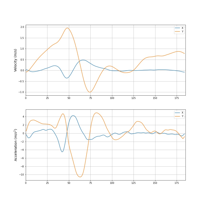
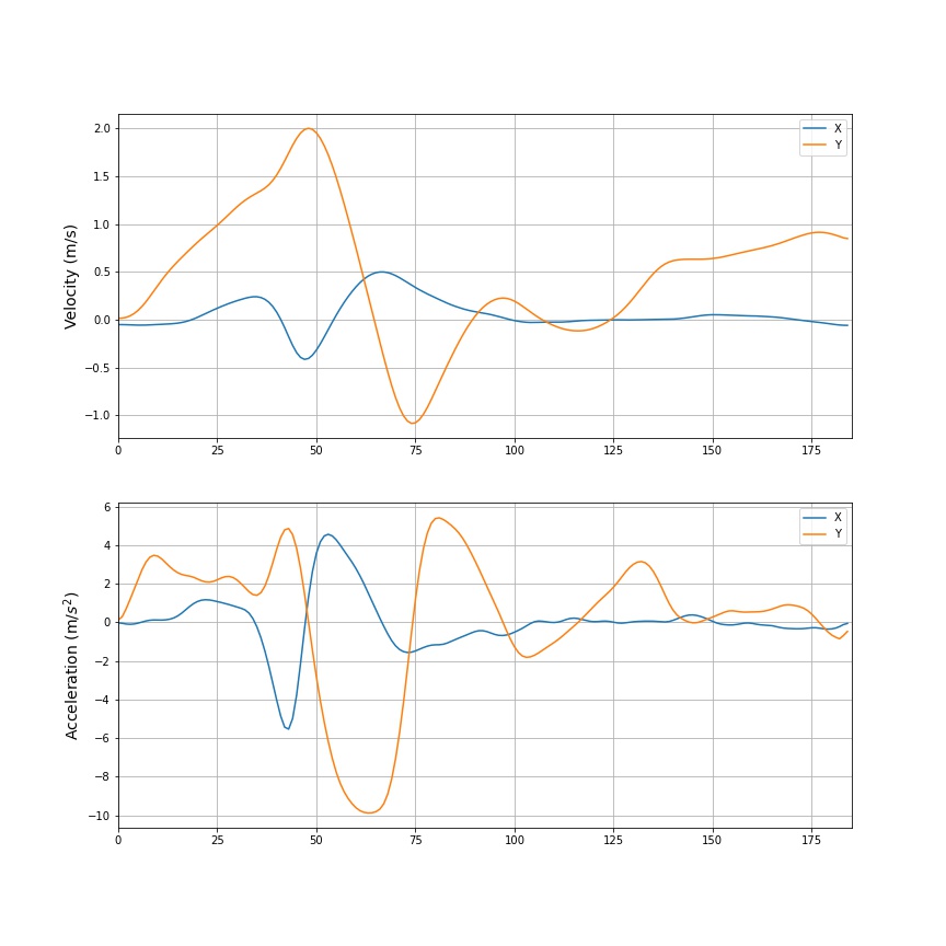
A great quality we see between the two graphs is that the peak values are very close in magnitude, even though the two cases use different tracking methods and were filtered at different frequencies. This is important for the repeatability and reliability of the metrics calculated from these time series but also shows that we aren’t compromising too much of the key signal with the filter. If we were filtering over-aggressively, we’d expect to see the key features of the curves smoothed out and the peaks of the lower frequency filtered plot to be significantly less in magnitude.
The residual analysis allows us to calculate the appropriate cutoff frequency for different movements over a variety of conditions. Not only does this allow us to collect reliable data regardless of circumstances but it also allows for the the tracking algorithms to be continually improved while also trusting the filtering will adjust dynamically to accommodate the new data characteristics.
Resources:
Winter, David A. Biomechanics and motor control of human movement. John Wiley & Sons, 2009.
